The problem
Map two square kilometres of Banff National Park in enough detail to plan trails and infrastructure, with minimal disturbance to the site.
The survey area contains three distinct terrain types: a stretch of the Bow River, forest on either side of it, and a mountainous section several hundred metres above the valley floor. Each places different demands on the survey. Forest requires enough returns to separate canopy from the ground beneath it. Water returns very little. Steep rock requires point density on faces that sit at a shallow angle to the aircraft.
The work covers sensor selection, aircraft selection, flight pattern design that maintains a usable standoff over terrain of varying height, and the regulatory case for operating an unmanned aircraft inside a national park.
Sensor selection
The sensor was selected before the aircraft. On a survey mission the sensor determines the data requirements, and the aircraft requirement follows from carrying it for the necessary duration.
The MNM LiDAR system weighs 730 g and combines a multi-return scanner with a tactical-grade inertial measurement unit and a multi-frequency GNSS receiver.
| Specification | Value | Effect on the survey |
|---|---|---|
| Pulse repetition | 240 kHz single, 480 kHz double, 720 kHz triple | Sets point density on the ground |
| Returns | Single first, single strongest, double, triple | Separates canopy from ground beneath it |
| Field of view | 70.4° horizontal × 4.5° vertical | Sets swath width and therefore line spacing |
| Beam divergence | 0.28° vertical × 0.03° horizontal | Keeps the spot tight at range |
| Roll and pitch | 0.04° RMSE | Attitude error propagates into point position |
| Heading | 0.13° RMSE | Same, increasing toward the swath edge |
| Gyro bias instability | 1.5°/hr | Limits heading drift over an hour-long flight |
| Positional accuracy | 0.01 m + 1 ppm CEP | Georeferences the point cloud |
| Mass | 730 g | Sets the aircraft payload requirement |
A LiDAR return provides a range and a direction. The range comes from the laser, but the direction depends on knowing the orientation of the aircraft at the instant the pulse was emitted. A tenth of a degree of attitude error at 100 m range corresponds to approximately 17 cm of position error on the ground, increasing toward the edges of a 70° swath. The inertial navigation system accuracy is therefore as significant as the laser specification.
Aircraft selection
The WingtraOne Gen II carries up to 800 g on a modular payload mount, leaving 70 g of margin over the sensor. It provides approximately one hour of flight time, sufficient to cover two square kilometres in a single sortie, and takes off and lands vertically before transitioning to fixed-wing flight.
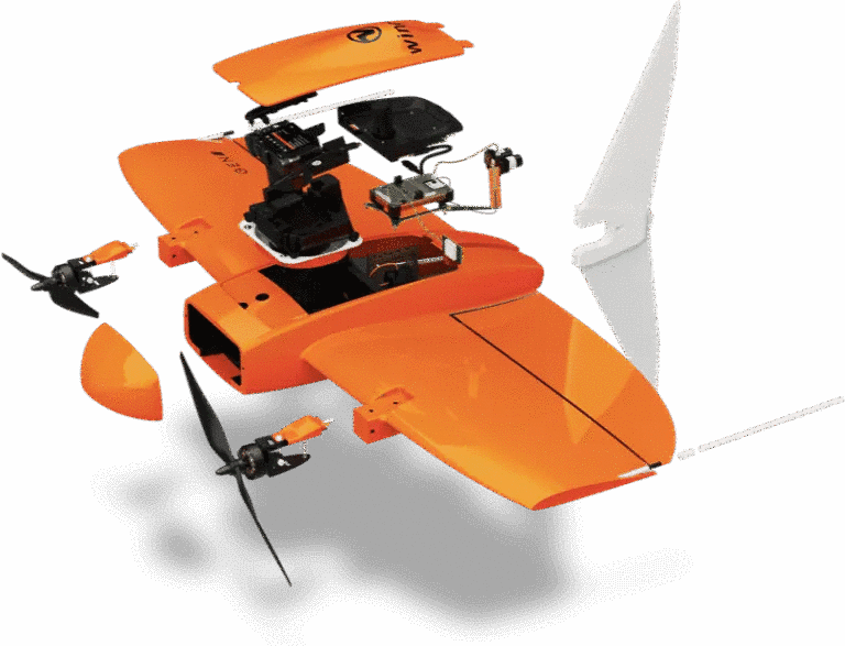
Both parts of the configuration are required for this mission. Vertical takeoff is necessary because the valley has no space for a conventional runway. Fixed-wing cruise is necessary because a multirotor could not cover the area within its endurance, and because a wing provides the stable platform a scanning LiDAR requires. Attitude noise appears directly in the point cloud, so airframe stability contributes as much to data quality as sensor specification.
The survey window is June to August, when average wind speed is between 1.61 and 2.1 m/s against an aircraft rated for 12 m/s sustained wind and 18 m/s gusts. The margin is kept wide because gusts displace the aircraft faster than the autopilot corrects, and those excursions appear in the data.
Survey patterns
The site was divided by terrain type and flown as two survey patterns at two altitudes, both within a single sortie.
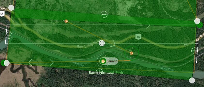
First pattern, river and forest
The valley floor is close to uniform, so it is surveyed with a zig-zag pattern at 90° with minimal overlap, held at 1,700 m above sea level, approximately 100 m above the terrain. Ground speed is 40 km/h, below the aircraft's normal cruise, because a slower pass increases pulse density on the ground and the fine structure of the forest and riverbank is the feature of interest.
Second pattern, mountainous section
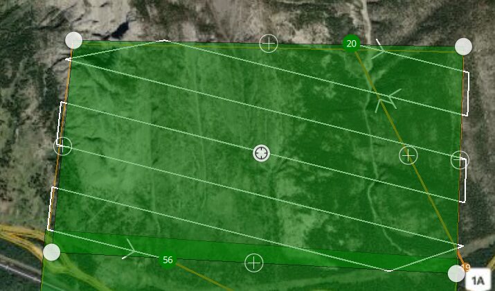
The mountainous section is surveyed at 2,230 m above sea level, again approximately 100 m above the terrain, at 30 to 35 km/h. Two aspects of the pattern were chosen deliberately.
The pattern starts at the far end near the peak and works back toward the base, where the launch site is located. Descending through the return leg rather than climbing is more battery efficient, which leaves reserve capacity at the end of the sortie. If a section returns poor coverage, there is enough remaining to resurvey it.
Ground speed is reduced to 30 to 35 km/h because uneven terrain requires higher point density than flat terrain. A rock face angled away from the aircraft receives pulses at shallow incidence and returns fewer of them, so reducing speed maintains density across the whole surface.
| Pattern 1 | Pattern 2 | |
|---|---|---|
| Terrain | River and forest | Mountainous |
| Altitude | 1,700 m ASL | 2,230 m ASL |
| Height above ground | ~100 m | ~100 m |
| Ground speed | 40 km/h | 30 to 35 km/h |
| Direction | Across the valley | Peak down to base |
The two absolute altitudes differ by 530 m while the height above ground is the same in both. This is the reason for splitting the site: a single-altitude survey would have been 100 m above one half and approximately 600 m above the other, and point density would have dropped substantially across the transition.
The aircraft completes the first pattern, climbs, transits to the peak and begins the second. Line spacing in both patterns was set by simulating the LiDAR field of view in STK and taking the swath width at the planned standoff, rather than by selecting an overlap percentage.
Data processing
Six steps convert the raw LiDAR data into terrain products usable for planning:
- Extract · transfer the data from the onboard card to a processing machine
- Clean · filter noise and remove returns not required for the surface being modelled, such as vegetation when modelling ground surface
- Classify · sort the point cloud into ground, forest, water and mountainous terrain
- Model · produce a digital elevation model for the mountainous section and a canopy height model for the forest
- Integrate · patch the data sets together and analyse the combined terrain to identify suitable ground
- Assess · plan trails and infrastructure against soil stability, vegetation cover and water bodies
The multi-return capability described in section 02 is what makes steps two and four possible. A first return from the canopy and a later return from the ground beneath it, from the same pulse, produces both a canopy height model and a bare-earth elevation model from a single flight.
Regulatory approvals
Operating in a national park requires two separate approvals from two different authorities.
The first is Transport Canada, which requires a Safety Assurance Integrity Level determination. Ground risk is derived from the kinetic energy of the aircraft:
This gives an intrinsic ground risk class of 4. The air risk class from the decision tree is ARC-c. Together these give a total of SAIL IV, a higher assurance burden than the SAIL II of the lake survey in project 04. The difference is driven by the operating environment rather than the aircraft.

The survey site is also close to a heliport and an airfield, so the operation requires the operator to remain in contact with both and exchange traffic information for the duration of the flight. This is a procedural mitigation and has to be included in the operating plan.
The second approval is a Restricted Activity Permit from the park Superintendent. This is separate from the aviation regulator and addresses whether the activity is acceptable within a protected area rather than whether the flight is safe.
Environmental considerations
Three measures support the permit application. Flights are scheduled to avoid nesting and migration periods, when disturbance has the greatest effect, and the WingtraOne produces minimal overhead flight noise. Flight paths are planned to minimise time spent over sensitive ecosystems. Sensor selection also contributes: a wide field of view and high precision reduces the number of survey lines required, shortening the flight and reducing total time over the park.
Imagery resolution
Covering the ground and being able to identify what is on it are separate questions, and the second one can be quantified.
The Johnson criteria relate the number of resolvable cycles across a target to the probability of detecting, recognising or identifying it. For a target 180 by 80 cm at a ground sample distance of 33 cm, the characteristic dimension and cycle count are:
| Task | N₅₀ | Probability |
|---|---|---|
| Detection | 0.75 | 98% |
| Recognition | 3.00 | 17.3% |
| Identification | 6.00 | 3.0% |
At this ground sample distance the imagery reliably establishes that an object is present, identifies its class correctly less than one time in five, and rarely identifies the specific object. A survey designed to locate objects and a survey designed to identify them require different resolution, and the difference is not addressed by additional flight time.
Limitations
This is a survey plan. No flight was conducted and no point cloud was produced.
Line spacing is derived from the sensor field of view simulated in STK at a nominal 100 m standoff. Real terrain does not hold a constant standoff between waypoints, so the actual swath varies along each line and the overlap margin is narrower in places than the plan assumes. A terrain-following altitude profile would correct this at the cost of a more complex flight plan.
Point density figures follow from the pulse repetition rate and ground speed, and assume returns are received. Water returns very little at these wavelengths and the Bow River is inside the survey area, so coverage over the river will be sparse in a way the plan does not model.
The environmental measures are stated rather than assessed. Scheduling around nesting and migration is the correct approach, but the specific species, dates and separation distances would require input from a park biologist and are not determined here.
This work formed part of a broader exam that also covered system reliability, aircraft state estimation and a lift-to-drag estimate. The lift-to-drag calculation returned 2.31 for a light single, which is too low to be correct and results from estimating both lift and drag coefficients from assumed reference values.