The target
ENVISAT was the largest civil Earth observation satellite ever flown, and it has been dead since 2012.
It launched in March 2002 and ESA lost contact with it on 8 April 2012. It weighs 8,211 kg, spans about 26 m with the solar array deployed, and sits in a sun-synchronous orbit near 790 km, which is one of the busier altitudes in low Earth orbit. Estimates put it up there for roughly another 150 years.
The problem is that nothing on it responds any more, so it cannot be moved out of the way of anything. If something does hit it, the debris ends up spread through an altitude band that a lot of other satellites are using.
Any mission that goes up to remove it needs a manipulator, and I wanted to work out what that manipulator has to do: choose a point on the satellite to grab and a direction to come in from, then find the angle each of the six joints needs to be at. The rest of the page works through that question.
I sized the arm on the Niryo One, which is a 500 mm educational robot, rather than on something that could actually handle eight tonnes. The kinematics do not depend on mass, so the same six transformation matrices apply whether the arm is half a metre long or fifteen. Working at a size where the manufacturer publishes real geometry meant I could check my answers against something instead of just trusting them.
Design of the manipulator
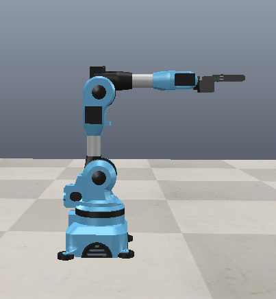
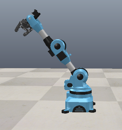
The arm is a serial chain. Six revolute joints with a link between each pair, the base fixed to the station, and a gripper on the far end. Nothing branches off, so each joint has to carry everything outboard of it, and the pose of the gripper is just the product of six transformations taken in order.
Two things about the layout matter more than the rest. The first is that the last three joint axes all pass through a single point, which makes the wrist spherical. I did that because it lets the inverse problem split into a position part and an orientation part that can each be solved directly. Without a spherical wrist you have to run a numerical solver at every waypoint, and then you still have to work out which of the several possible answers it landed on.
The second is that the joints do not have equal travel and none of them are symmetric about zero.
| No. | Link | Parent | Joint | Type | Travel | Range |
|---|---|---|---|---|---|---|
| 1 | Link 1 | Base | Joint 1 | Revolute | −175° to 175° | 350° |
| 2 | Link 2 | Link 1 | Joint 2 | Revolute | −90° to 36.7° | 126.7° |
| 3 | Link 3 | Link 2 | Joint 3 | Revolute | −80° to 90° | 170° |
| 4 | Link 4 | Link 3 | Joint 4 | Revolute | −174° to 175° | 349° |
| 5 | Link 5 | Link 4 | Joint 5 | Revolute | −100° to 110° | 210° |
| 6 | End effector | Link 5 | Joint 6 | Revolute | −147.5° to 147.5° | 295° |
Joint 2 is the shoulder and it is the most restricted joint on the arm. It has 126.7° of travel where the base has 350°, and only 36.7° of that is forward of vertical. In practice this limit sets the shape of the reachable workspace far more than the link lengths do. I had to move the capture point in twice before the shoulder could reach it, and even now it ends up within 8° of the stop.
Forward kinematics
Forward kinematics means going from a set of joint angles to the position and orientation of the gripper. It is the easier of the two directions, and it is also what I check everything else against.
The Denavit-Hartenberg convention describes the relationship between two consecutive links using four parameters, and only four, which is the reason it is worth using at all:
- ai · length of the link along the common normal
- αi · twist from the old z axis to the new one about that normal
- di · offset along the previous z axis to the common normal
- θi · joint angle about the previous z axis, from the old x axis to the new one
Each row of four gives you one transformation matrix:
Multiplying all six together gives the transformation from the base frame to the gripper:
These are the parameters the arm runs on. Three of the a values come out at zero, which is what you get when the frames are assigned sensibly.
| i | ai (m) | αi | di (m) | θi offset | |
|---|---|---|---|---|---|
| 1 | 0 | −90° | 0.103 | 0 | base to shoulder |
| 2 | 0.210 | 0 | 0 | −90° | upper arm |
| 3 | 0.0415 | −90° | 0 | 0 | elbow offset |
| 4 | 0 | 90° | 0.180 | 0 | forearm to wrist centre |
| 5 | 0 | −90° | 0 | 0 | wrist |
| 6 | 0 | 0 | 0.0237 | 0 | wrist centre to tool tip |
Rows 4, 5 and 6 all have ai = 0, which is the spherical wrist written out. The three axes meet at the origin of frame 4, and the only thing between that point and the tool tip is a 23.7 mm offset along the tool’s own z axis. Section 04 uses that.
Inverse kinematics
Inverse kinematics is the direction you actually need for planning. You know where you want the gripper and which way you want it pointing, and you have to work backwards to the six joint angles.
Because the wrist is spherical this splits cleanly in two. The position of the gripper is set almost entirely by the first three joints and its orientation by the last three, so the two halves can be solved one after the other rather than together.
Inverse position problem
If you back the tool tip off along its own z axis by the 23.7 mm from the table, you arrive at the wrist centre, which is the one point on the arm that the last three joints cannot move:
Joint 1 comes directly from where that point sits in plan view. Joints 2 and 3 are then a planar two-link problem in the vertical plane joint 1 has just swept out, with the shoulder at one end and the wrist centre at the other.
The forearm is not a straight link, and this is easy to get wrong. There is a 41.5 mm offset at the elbow and then 180 mm out to the wrist centre, so the effective link is 184.7 mm long and it sits 12.98° off the line you would draw between the two joints. If you ignore that, every solution comes back a couple of centimetres short, and the error looks like a rounding problem rather than a geometry problem.
Inverse orientation problem
Once the first three angles are known, the rotation they produce is known as well, so you can take it off the target and whatever is left is what the wrist has to supply:
I take R30 from the forward kinematics pass rather than deriving it separately. If you derive the same rotation twice you have two things that can disagree with each other, and when they do the symptom is a pose that is a few degrees off with nothing obviously wrong in either derivation.
Choosing between the solutions
Any reachable pose has eight solutions: elbow up or down, shoulder reaching forwards or leaning back over the base, and the wrist folded either way. All eight put the gripper in the same place, but they are not interchangeable.
So the solver works out all eight and ranks them. Joint limits come first, since a solution that breaks a stop is not a solution. After that it ranks on how far each one sits from the previous waypoint. Two waypoints only a few centimetres apart can easily be solved on different branches, and if you then interpolate between them the arm swings through most of its workspace and comes back. The joint angles are valid at both ends; the path between them is not, because the elbow sweeps through the payload on the way.
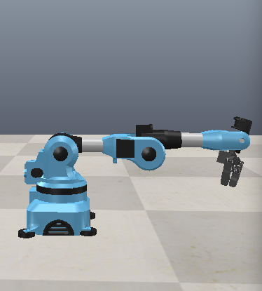
There is a related problem at the wrist. When joint 5 passes through zero the axes of joints 4 and 6 line up, only their sum is determined by the target, and the solver is free to return any split that adds up to it. My first version of the capture approach ran almost straight into that. Joint 4 came back at −50° at the capture waypoint against +6° at the waypoint 40 mm before it, and both were correct as poses. The interpolation between them was not. The fix was to search the approach direction rather than to patch the angles afterwards, because a couple of degrees of joint 5 is enough to make the two splits genuinely different orientations. The approach the arm uses now comes down at 74° below horizontal and keeps joint 5 about 55° clear of zero the whole way in.
Checking the solver is straightforward once you trust the forward direction. I generate 3,000 random joint configurations inside the limits, run forward kinematics on each to get a pose, hand that pose back to the solver, and compare what comes out. The worst position error over the run was 5×10⁻¹⁶ m.
Path planning
A capture is a sequence of poses rather than a single one, and the arm has to be somewhere sensible at every point in between.
Waypoints are specified as homogeneous transforms, which pack a rotation and a translation into one matrix, so each waypoint says both where the gripper goes and which way it faces:
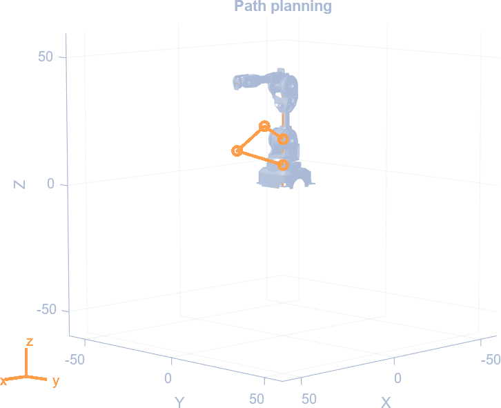
Each waypoint goes through the inverse solver once. After that the arm is described by six numbers per waypoint, and the path between them is interpolated:
I interpolate in joint space and the reason is the joint limits. The limits are a box, six independent intervals, and a straight line between two points inside a box stays inside the box. So if both waypoints are legal then everything between them is legal as well, and there is nothing left to check. Interpolating the gripper along a straight line in space gives you no such guarantee, and you end up testing the limits at every sample and backing off whenever one trips.
What it costs is that the tip does not travel in a straight line, it bows out slightly. That is why standoff, approach and capture are three separate waypoints along one line rather than a single long move. Over the last 40 mm the bow is small enough to ignore, and the gripper goes in along the axis of the post instead of sliding sideways across it.
| Waypoint | J1 | J2 | J3 | J4 | J5 | J6 |
|---|---|---|---|---|---|---|
| Stowed | 0.0 | −56.0 | 66.0 | 0.0 | −16.0 | 0.0 |
| Standoff | −26.0 | 24.8 | −37.5 | 0.0 | 86.7 | −116.9 |
| Approach | −26.0 | 25.3 | −16.5 | 0.0 | 65.2 | −116.9 |
| Capture | −26.0 | 28.9 | −9.9 | 0.0 | 55.1 | −116.9 |
| Lift | −26.0 | 27.1 | −48.0 | 0.0 | 94.9 | −116.9 |
| Berth | 78.0 | 19.3 | −21.8 | 0.4 | 61.8 | −115.8 |
All in degrees. Joint 2 is the one to watch at capture, 28.9° against a 36.7° stop. Joint 1 holds at −26° through all four approach waypoints because the approach runs along a single line and the base does not have to turn to follow it, then it does 104° on its own during the carry. Joint 6 does not move at all through the approach, which is what you get by solving the four collinear waypoints on one shared tool roll instead of letting each one choose its own.
Limitations
All of the above is kinematics. There is no mass anywhere in it.
The model stops there. The arm knows what angles its joints need to be at and nothing about what it costs to get to them. No inertias, no joint torques, no reaction back into the station, no contact model at the gripper. For a half-metre arm on a bench that is a reasonable thing to leave out. For eight tonnes of tumbling satellite it is the part that decides whether the capture works at all, because as soon as the gripper closes the arm and the debris are one body and whatever angular momentum ENVISAT had becomes the station’s problem.
There are two smaller gaps as well. Interpolating in a straight line through joint space means every joint runs at a constant rate and then reverses direction instantly at each waypoint, which no real actuator will do. Putting a trapezoidal or S-curve velocity profile over the same joint path would fix that without changing anything above it. And nothing here checks the arm against itself or against the payload. The branch continuity rule in section 04 avoids the obvious collisions by keeping consecutive waypoints in the same family of solutions, which reduces the risk without checking it.
The original MATLAB and the CoppeliaSim scene are both lost. The parameters in section 03 came back out of the manufacturer’s published geometry, and I rewrote the kinematics from scratch and checked them against themselves, which is why section 04 quotes a round-trip residual rather than showing a screenshot. The simulation figures are from the original work.