Slingshot to L1 | Anshuman Vyas

The mission

Aditya-L1 is India's first dedicated solar observatory. It carries seven payloads: four looking directly at the Sun, three measuring particles and fields in situ. It launched on 2 September 2023.

L1 is used instead of an Earth orbit because the view of the Sun is uninterrupted. A spacecraft near the first Sun-Earth Lagrange point sees the Sun continuously, with no occultation by the Earth, so coronal mass ejections and flare activity can be observed as they develop.

This project reproduces that trajectory from the ground up: establish the parking orbit, raise it in stages, escape Earth's sphere of influence, find L1 numerically, pick a halo orbit around it, and patch the two halves of the journey together.

The parking orbit

The spacecraft is first placed in an elliptical orbit with a perigee radius of 235 km and an apogee radius of 19,500 km, inclined 19.2°, with an argument of perigee of 346.6°. Perigee velocity comes from the vis-viva equation:

v_p = \sqrt{\mu\left(\frac{2}{r_p} - \frac{1}{a}\right)} μ is Earth's gravitational parameter, rₚ the perigee radius, a the semi-major axis.

Velocity at perigee is tangential, so in the perifocal frame the state is simply r = [rₚ, 0, 0] and v = [0, vₚ, 0]. Orienting that into the correct plane is two rotations, one for inclination and one for the argument of perigee:

R_i = \begin{bmatrix} 1 & 0 & 0 \\ 0 & \cos i & -\sin i \\ 0 & \sin i & \cos i \end{bmatrix} \qquad R_\omega = \begin{bmatrix} \cos\omega & -\sin\omega & 0 \\ \sin\omega & \cos\omega & 0 \\ 0 & 0 & 1 \end{bmatrix} Applied to both the position and velocity vectors to give the oriented parking orbit.

Raising the orbit

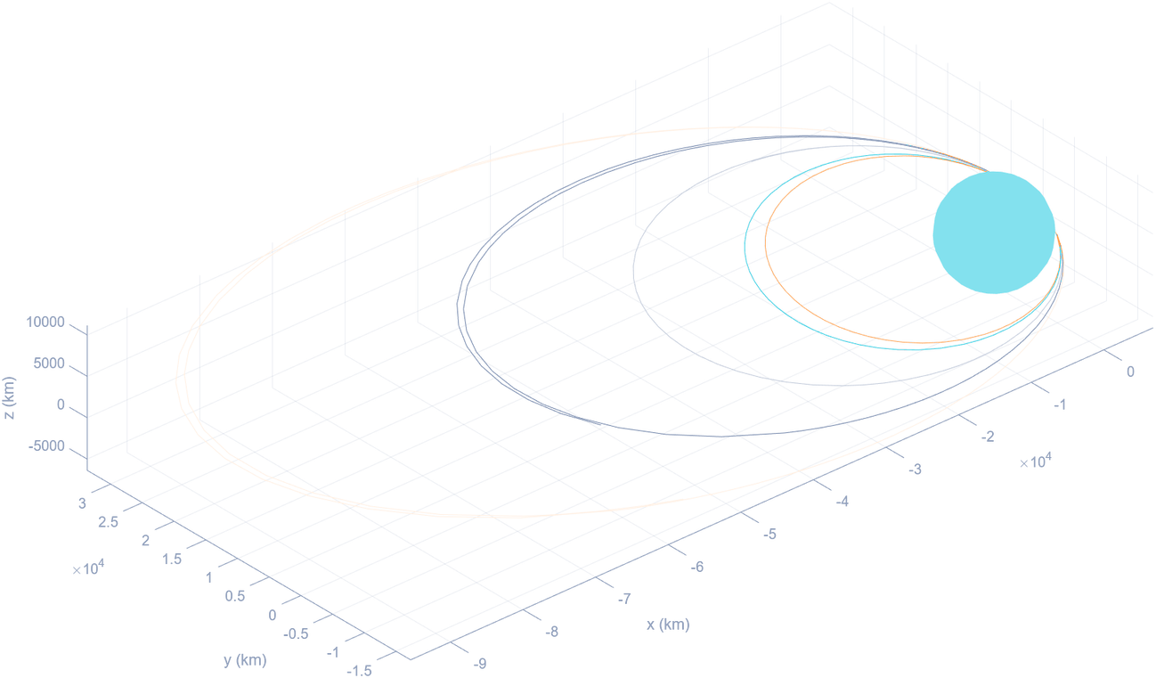
Indian launch vehicles cannot give a spacecraft escape velocity directly, so the orbit is built up instead. This is the slingshot technique, and it works because of the Oberth effect, which states that the most efficient place for a spacecraft to change velocity is at the lowest point of its orbit. For an elliptical orbit that is the perigee.

The same burn point is used four times, each burn raising the apogee further:

Stage	Perigee	Apogee
Initial	235 km	19,500 km
Burn 1	245 km	22,459 km
Burn 2	282 km	40,225 km
Burn 3	296 km	71,767 km
Burn 4	256 km	121,973 km

\Delta V = V_{p2} - V_{p} Vₚ₂ is the perigee velocity required to hold the larger orbit, found from the same vis-viva expression with the new semi-major axis.

Five nested elliptical orbits around Earth, each larger than the last — **Figure 1 · Orbit raising** The parking orbit and the four raised orbits, plotted together in the Earth-centred frame. Each burn is applied at the same physical point, so all five ellipses share a perigee.

Escaping Earth’s sphere of influence

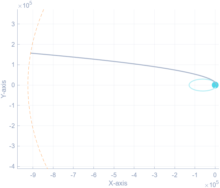
To escape a planet's gravity the spacecraft has to be on a hyperbolic trajectory relative to it, arriving at the edge of the sphere of influence with hyperbolic excess velocity greater than zero:

v_\infty = \sqrt{\frac{\mu_{\odot}}{R_1}}\left(\sqrt{\frac{2R_2}{R_1 + R_2}} - 1\right) R₁ is the Sun-Earth distance, R₂ the Sun-L1 distance, μ_☉ the Sun's gravitational parameter.

That fixes the velocity needed at the periapsis of the hyperbola, and the fifth and final burn is the difference between it and the speed the spacecraft already has there:

V_{ph} = \sqrt{v_\infty^{2} + \frac{2\mu}{r_p}} \qquad \Delta V = V_{ph} - V_{pf} Applied at the perigee of the final raised orbit, as with the four before it.

Trajectory leaving Earth on a hyperbolic path toward the edge of the sphere of influence — **Figure 2 · Escape** The hyperbolic departure from the final parking orbit out to the edge of Earth's sphere of influence, where the two-body Earth problem stops applying.

Locating L1

Lagrange points are the positions where the gravitational pull of two large bodies supplies exactly the centripetal force a small third body needs to move with them. There are five. The three collinear ones lie on the line joining the two masses and all three are unstable. L1 currently hosts SOHO; L2 hosts JWST.

Locating them means working in the circular restricted three-body problem. In the rotating, non-dimensional frame the equations of motion are:

\begin{aligned} \ddot{x}^{*} - 2\dot{y}^{*} - x^{*} &= -\frac{1-\pi_2}{\sigma^3}(x^{*}+\pi_2) - \frac{\pi_2}{\psi^3}(x^{*}-1+\pi_2) \\ \ddot{y}^{*} + 2\dot{x}^{*} - y^{*} &= -\frac{1-\pi_2}{\sigma^3}y^{*} - \frac{\pi_2}{\psi^3}y^{*} \\ \ddot{z}^{*} &= -\frac{1-\pi_2}{\sigma^3}z^{*} - \frac{\pi_2}{\psi^3}z^{*} \end{aligned} π₂ = m₂ / (m₁ + m₂). σ and ψ are the distances to the two primaries.

In this form the equations depend only on the mass ratio μ. They do not depend on the two masses individually, on the rotation rate of the frame, or on the separation between the primaries. The same equations therefore describe the Sun-Earth and Earth-Moon systems.

At an equilibrium point every velocity and acceleration term vanishes. Setting y* = 0 for the collinear case leaves a single equation in x*:

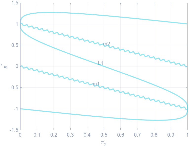
x^{*} - \frac{1-\pi_2}{|x^{*}+\pi_2|^{3}}(x^{*}+\pi_2) - \frac{\pi_2}{|x^{*}-1+\pi_2|^{3}}(x^{*}-1+\pi_2) = 0 Quintic in x*. No closed-form solution, so it is solved numerically.

Plot of the collinear Lagrange point equation showing S-shaped curve with roots — **Figure 3 · Collinear roots** The collinear condition plotted. Solutions lie on the S-shaped curve; L1 is the root between the two primaries.

With the Sun-Earth distance normalised to 1 AU, the solver puts L1 at x* = 0.9900, one percent of the way back from Earth toward the Sun. At 1 AU ≈ 150 million km, that is roughly 1.5 million km from Earth.

Selecting the halo orbit

Linearising the equations of motion about L1 and solving for small departures shows it to be a saddle point, which is dynamically unstable. A spacecraft left at the point drifts away from it, so Aditya-L1 is placed in an orbit around L1 rather than at the point itself.

The halo orbit is selected by its out-of-plane amplitude A_z, which can range from zero up to about 920,000 km. Larger halos have a communications penalty, so an intermediate A_z = 120,000 km was chosen.

Richardson's method gives the starting approximation, a linearised periodic solution about the libration point:

\begin{aligned} x &= -A_x\cos(\lambda t + \phi) \\ y &= kA_x\cos(\lambda t + \phi) \\ z &= A_z\cos(\lambda t + \psi) \end{aligned} A_x and A_z are not independent: a nonlinear algebraic constraint from the perturbation method links them, and the phases φ and ψ are linearly related.

The orbit only closes when the amplitudes are large enough for the nonlinear terms to bring the in-plane and out-of-plane eigenfrequencies into agreement. Below that they stay mismatched and the motion is a Lissajous figure, which never quite repeats.

Richardson’s solution is linearised, so what it produces is close to a halo orbit without being one. That is enough to choose an amplitude and see the shape, and it is where the report stopped. Turning it into an orbit that actually repeats is section 08.

Three-dimensional plot of the halo orbit looping around the L1 point — **Figure 4 · Richardson’s approximation** The halo orbit as the linearised solution gives it, at A_z = 120,000 km. The marker at the centre is the libration point itself, which the spacecraft never occupies. This is a starting guess rather than a periodic orbit. Propagated in the full nonlinear problem it does not close, which is what section 08 fixes.

Transfer to L1

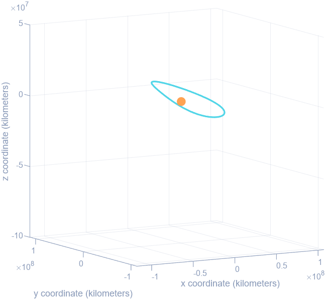
The journey is stitched together with the patched conic method: two separate two-body problems joined at the boundary of Earth's sphere of influence. Inside it, the spacecraft is on a hyperbola about Earth. Outside it, the assumption is that it follows an unperturbed Keplerian orbit about the Sun.

Crossing that boundary is a change of frame. The spacecraft has been carrying Earth's orbital motion around the Sun the whole time it was in the parking orbit, so both position and velocity get Earth's added to them:

\begin{aligned} \mathbf{r}_{sat,\odot} &= \mathbf{r}_{sat,\oplus} + \mathbf{r}_{\oplus} \\ \mathbf{v}_{sat,\odot} &= \mathbf{v}_{sat,\oplus} + \mathbf{v}_{\oplus} \end{aligned} Earth-centred state to heliocentric state at the sphere-of-influence crossing.

With the spacecraft and L1 both expressed heliocentrically, the transfer arc between them is a Lambert problem: given two position vectors and a time of flight, find the orbit that connects them. A universal-variable Lambert solver returns the velocities required at both ends, and the total cost of the transfer is the sum of two impulses.

\Delta V_{total} = \Delta V_1 + \Delta V_2 ΔV₁ departs the sphere of influence onto the transfer arc. ΔV₂ is what it costs to stay once there.

Why ΔV₂ is not zero

At L1 exactly, an idealised spacecraft needs nothing to stay in place, since it is an equilibrium point and the required velocity is zero. In practice L1 is unstable and the halo orbit has to be actively maintained. Station-keeping works out to roughly 0.2 to 0.4 m/s, and that is what sets ΔV₂.

Halo insertion

The halo orbit in section 06 comes from Richardson’s linearised solution, which is an approximation to a periodic orbit rather than a periodic orbit itself.

Propagated in the full nonlinear CR3BP it does not close, because the terms the linearisation drops are the ones that make the orbit periodic. Closing it is a separate numerical problem, and the rest of this section is how it was solved.

Linearising about L1

The first step is linearising about L1, done numerically rather than by transcribing a closed-form Jacobian. Central differences on the equations of motion give the 6×6 Jacobian at the equilibrium state:

J_{ij} = \frac{f_i(\mathbf{s}_{L1} + h\mathbf{e}_j) - f_i(\mathbf{s}_{L1} - h\mathbf{e}_j)}{2h}, \qquad h = 10^{-7} f is the CR3BP vector field, s_L1 the equilibrium state [x_L1, 0, 0, 0, 0, 0].

Eigendecomposing the planar submatrix in (x, y, v_x, v_y) gives a real unstable pair and a purely imaginary pair. The imaginary pair is the in-plane oscillatory mode, λ_xy = 2.0864, and its eigenvector gives the direction the seed should point.

Choosing the seed amplitude

The corrector below builds its Jacobian by perturbing x₀ by 10⁻⁶, which is about 150 km. If the eigenvector is scaled down to a seed of similar size, the perturbation is as large as the orbit itself, the finite difference measures nothing useful, and Newton diverges within three iterations. Seeding at around 10⁵ km, which is the amplitude the orbit will actually have, keeps the perturbation at a tenth of a percent of the state and the corrector converges in six iterations.

Differential correction

Halo orbits are symmetric about the x-z plane, which is what allows a two-variable shooting method. The trajectory starts on the plane, moving perpendicular to it:

\mathbf{s}_0 = [\,x_0,\; 0,\; z_0,\; 0,\; \dot{y}_0,\; 0\,]^{\mathsf{T}} Four of the six components are fixed by the symmetry. Only x₀ and ẏ₀ are free.

If the orbit is periodic, then propagating half a revolution to the next y = 0 crossing must arrive perpendicular to the plane again, which means both remaining velocity components vanish there. That is two residuals for two unknowns, solved by a 2×2 Newton step:

\begin{bmatrix} \Delta x_0 \\ \Delta \dot{y}_0 \end{bmatrix} = -J_c^{-1}\begin{bmatrix} \dot{x}_h \\ \dot{z}_h \end{bmatrix}, \qquad J_c = \begin{bmatrix} \dfrac{\partial \dot{x}_h}{\partial x_0} & \dfrac{\partial \dot{x}_h}{\partial \dot{y}_0} \\[6pt] \dfrac{\partial \dot{z}_h}{\partial x_0} & \dfrac{\partial \dot{z}_h}{\partial \dot{y}_0} \end{bmatrix} Subscript h denotes the state at the half-period crossing. J_c is built by finite differences, and the step is damped early in the iteration to keep it stable.

The event that stops the integration is the y = 0 crossing itself, detected by the ODE solver rather than by stepping and checking, so the half-period comes out to integrator precision instead of step size.

Amplitude continuation

Going straight to the target amplitude would ask Newton to converge from well outside its basin, so the amplitude is walked up instead. A_z steps from 2,000 km to 120,000 km over sixty increments, with the corrector re-converging at each one and each solution seeding the next.

Why the tolerance is 10⁻⁹

The corrector's Jacobian is built by finite differences with a step of 10⁻⁶, on trajectories integrated to a relative tolerance of 3×10⁻¹³. That puts a noise floor of roughly integrator tolerance over step size on the Jacobian itself. Asking for a residual tighter than that noise does not improve accuracy; it stalls the iteration short of the target. 10⁻⁹ sits above the floor and still corresponds to a position error on the order of centimetres.

Verifying the orbit

Convergence of the corrector does not by itself prove that the orbit closes, so the converged state is propagated one full period at tight tolerance and compared with where it started:

T = 2t_{1/2}, \qquad \varepsilon = \left\lVert \mathbf{r}(T) - \mathbf{r}(0) \right\rVert d d is the Sun-Earth distance, converting the non-dimensional closure error back into kilometres.

Quantity	Value
x₀	0.988882, i.e. 171,200 km sunward of L1
z₀	0.000802, A_z = 120,000 km as targeted
ẏ₀	+0.008902
Period	3.0598 non-dimensional = 177.9 days
Closure error	0.228 km in position over one full period
Insertion ΔV	265.1 m/s
Drift, 5 periods	1.45 × 10⁷ km, no station-keeping

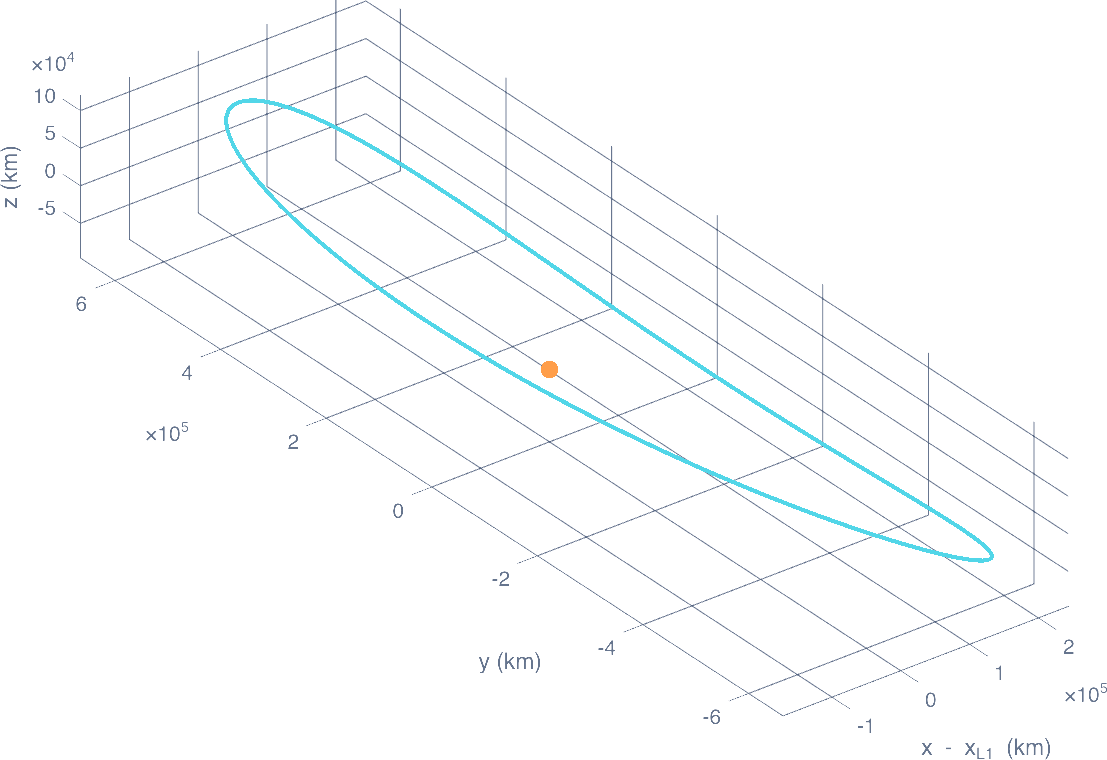
Three-dimensional plot of the converged halo orbit, a long inclined loop around the L1 point — **Figure 5 · The corrected orbit** The same orbit after differential correction, propagated one full period. Unlike Figure 4 this one closes, to within 228 m. It starts 171,200 km sunward of L1, stands 120,000 km out of the ecliptic and runs 665,000 km to either side of the Sun-Earth line. Axes in km, relative to L1.

One revolution takes just under six months. The insertion figure is the speed the spacecraft needs on arrival, measured against a vehicle at rest at that point in the rotating frame. Holding the orbit afterwards costs extra.

Propagating without station-keeping

The last check propagates the converged orbit for five full periods with nothing applied to hold it. It closes to within 228 m over the first period and ends up 14.5 million km from where it started by the fifth.

The divergence is physical rather than numerical. L1 is a saddle point and the halo orbit around it inherits that instability, so the error grows exponentially: under a kilometre after one revolution and a tenth of an AU after five. The exact five-period figure also depends on the integrator. Swapping ode113 for a Dormand-Prince scheme moves it by a factor of four, because an orbit this unstable amplifies whatever it is given, including rounding.

This is what the 0.2 to 0.4 m/s from section 07 pays for. Without it, the orbit follows that drift all the way out.

Replay the insertion on its own ↗

← All selected work Get in touch →